Protein-ligand interactions overlay

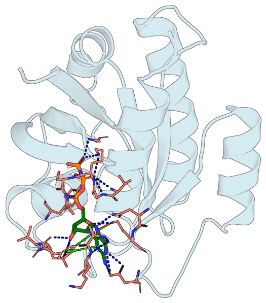
Detect hydrogen bonds, salt bridges, π-cation, and π-stacking interactions between a protein and its bound ligand (using peppr), and render them as colored dashed lines over a ray-traced cartoon — H-bonds in blue, salt bridges in yellow, π-cation in orange, π-stacking in green (parallel) or smudge (T-shaped), following PLIP’s conventions.

import tempfile
from pathlib import Path

import matplotlib.pyplot as plt
import yaml
from biotite import structure as struc
from PIL import Image

import portein

# Send PyMOL renders to a tempdir so they don't clutter the notebook dir.
output_dir = Path(tempfile.mkdtemp())

Load the structure and split receptor/ligand

PDB files don’t carry CONECT records by default, so we add bonds via biotite’s residue- template lookup before splitting into receptor and ligand.

pdb = portein.read_structure("../_data/7lc2.pdb")
chain_a = pdb[pdb.chain_id == "A"]
chain_a.bonds = struc.connect_via_residue_names(chain_a)

ligand = chain_a[chain_a.res_name == "GNP"]
receptor = chain_a[chain_a.res_name != "GNP"]

Detect interactions

With rotate=True, we orient the receptor + ligand so the 2D projection maximizes the spread of the interaction atoms — usually a better view of the binding pocket than the default protein-area maximization in ProteinConfig.

interactions = portein.InteractionSet.find(receptor=receptor, ligand=ligand, rotate=True)

print(f"H-bonds: {len(interactions.hbonds)}")
print(f"Salt bridges: {len(interactions.salt_bridges)}")
print(f"π-cation: {len(interactions.pi_cation)}")
print(f"π-stacking: {len(interactions.pi_stacking)}")

[16:53:18] Can't kekulize mol.  Unkekulized atoms: 22 23 24 27 28 30 31
[16:53:18] Can't kekulize mol.  Unkekulized atoms: 22 23 24 27 28 30 31

/home/runner/work/portein/portein/portein/rotate.py:23: NumbaPerformanceWarning: np.dot() is faster on contiguous arrays, called on (Array(float64, 1, 'A', False, aligned=True), Array(float64, 1, 'A', False, aligned=True))
  m = find_best_projection(coords)
/home/runner/work/portein/portein/portein/rotate.py:23: NumbaPerformanceWarning: np.dot() is faster on contiguous arrays, called on (Array(float64, 2, 'C', False, aligned=True), Array(float64, 1, 'A', False, aligned=True))
  m = find_best_projection(coords)
/home/runner/work/portein/portein/portein/rotate.py:28: NumbaPerformanceWarning: np.dot() is faster on contiguous arrays, called on (Array(float64, 2, 'A', False, aligned=True), Array(float64, 2, 'F', False, aligned=True))
  matrix = rotate_to_maximize_bb_height(coords[:, :2]) @ matrix

H-bonds: 20
Salt bridges: 0
π-cation: 1
π-stacking: 2

Render with the interactions overlaid

Pass the InteractionSet to Pymol(interactions=...). The render adds one PyMOL cmd.distance per interaction (with PLIP colors) and creates a named selection portein_interaction_residues that any layer can target — typically a thin-stick rendering of the participating side chains so the dashes have visible atoms to terminate at.

with open("../../configs/pymol_settings.yaml") as f:
    pymol_settings = yaml.safe_load(f)

protein_config = portein.ProteinConfig(
    pdb_file=interactions.combined,
    rotate=False,
    width=700,
    chain_to_color={"A": "lightblue"},
    output_prefix=str(output_dir / "interactions"),
)

image_file = portein.Pymol(
    protein=protein_config,
    layers=[
        # Protein as cartoon in backdrop
        portein.PymolConfig(
            representation="cartoon",
            pymol_settings=pymol_settings,
            selection="all",
            transparency=0.5,
        ),
        # Interacting residues and ligand as sticks
        [
            portein.PymolConfig(
                representation="sticks",
                pymol_settings={**pymol_settings, "stick_radius": 0.15},
                selection="portein_interaction_residues",
                color="salmon",
            ),
            portein.PymolConfig(
                representation="sticks",
                pymol_settings={**pymol_settings, "stick_radius": 0.25},
                selection="resn GNP",
                color="green",
            ),
        ],
    ],
    # Interactions as dashed lines
    interactions=interactions,
).run()

Crop and display

cropped = portein.crop_to_content(Image.open(image_file))
DPI = 100
fig, ax = plt.subplots(figsize=(cropped.width / DPI, cropped.height / DPI), dpi=DPI)
ax.imshow(cropped)
ax.axis("off")
fig.subplots_adjust(left=0, right=1, top=1, bottom=0)
plt.show()